1. Introduction

While the sliding of large masses of snow is called an 'Avalanche' - a topic that I've covered previously, the sliding of rock, debris, earth or soil is termed as a 'Landslide' - a phenomena which impacts us more often, quite literally.
Both these hazards are a form of Mass wasting - a down-slope movement of material under the influence of gravity. Mudslides - a liquefied and faster debris and dirt flow - is another type of Mass wasting and is highly devastating too.
Initially developed by geologist David Varnes in 1978 and subsequently refined by several researchers over time, Landslides can be classified as per their type of movement under six broad categories: Fall, Topple, Slide, Spread, Flow and Slope Deformation (Figure 1)
Section Hyperlinks:
India encounters several Landslide incidents - 61 have been recorded within the first 8 months of 2021 itself. The vicious slant of Slope and the pull of Gravity are essentially the key influencing factors of Landslides. Rainfall, Loose Soil, Ground Deformation also contribute towards the formation of this hazard. The Geological Survey of India (GSI), a scientific agency operated by the government, indicates that 'about 0.42 million sq. km or 12.6% of land area, excluding snow-covered area, are prone to landslide hazard' - an astounding threat.
Landslide Hazard Analysis & Mapping workflows involve the use of surface datasets such as terrain, slope and other influencing parameters obtained from topographic, aerial and remote sensing mediums which are subsequently processed on geospatial platforms (GIS) to identify locations which are susceptible to Landslide. GSI has created-
a) region-specific Landslide forecasting models using Rainfall and Land Slope as its main variables &
b) site-specific Landslide Forecasting models using advanced scientific instruments at eight sites in India currently. As per GSI, 90% of the landslides occurring in India is linked to rainfall - hence, this variable is given extra weightage in their predictive models.
In this post, I will demonstrate 3 Landslide workflows a) Creating a Landslide Risk Model b) Identifying at-risk Stakeholders and Infrastructure using a Landslide Risk Model and c) Rapid Detection of Landslide location using Radar Satellite Imagery. These would help you obtain an end-to-end picture of the subject matter as well as understand the capabilities of modern geotechnology.
You may view a demonstration of all the three workflows from the video below-
Video 1: Mapping & Analyzing Landslide Hazard using powerful Location Analytics platforms
2. Creating a Landslide Risk Model
Landslide Risk models need to be re-evaluated after major events such as earthquakes, wildfires, heavy rainfall etc. because the terrain / surface characteristics tend to change after such events making certain areas more susceptible to Landslides. In this workflow, I will demonstrate the creation of a new Landslide Risk Model after the occurence of a wildfire in the study area.
Much thanks to Learn ArcGIS for the training resources
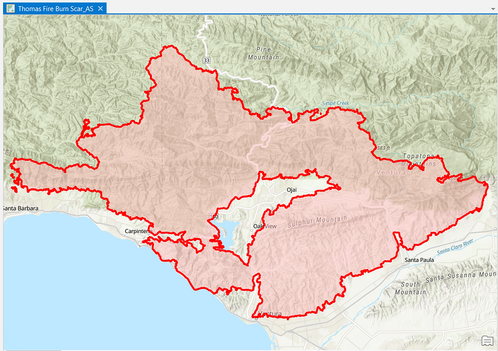
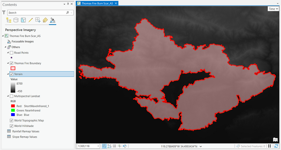
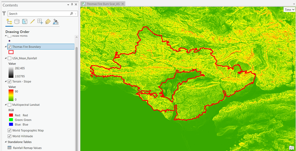


Now that I have all the necessary layers for the Risk Model loaded onto the GIS software, I will proceed to create a Geoprocessing Chain as depicted in the image below. This is essentially the technical procedure i.e. the 'methodology' used to generate the Risk Model. Instead of running one command at-a-time, I'll run this graph of sequential commands (Figure 7 below) which will automatically proceed to generate the final output at the click of a button.
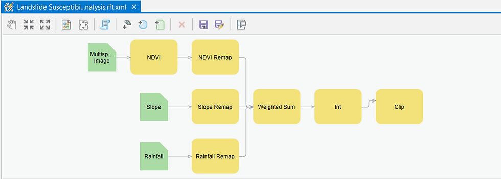
So what does the processing steps constitute?
At first, the GIS software will compute and convert the Multispectral Satellite Imagery layer into a Normalized Difference Vegetation Index (NDVI) layer. NDVI helps to delineate which surface features have more chlorophyll i.e. the presence of healthy vegetation from those which have less / no chlorophyll (unhealthy vegetation, urban areas, barren land etc.). This Vegetation Density information is a vital component of the Risk Model as dense vegetation holds the Soil together whereas sparse or no Vegetation makes the Soil more susceptible to breaking-up i.e. more vulnerable to Landslides.
The Remap processing steps applied to all the three layers helps to 'classify' the pixel values into distinct categories.

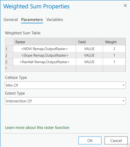
The Weighted Sum part of the processing chain allows me to combine the pixel values of all the three Remapped layers into a new weighted value output layer.
In the model that I'm working on, I've assigned the NDVI layer a higher weightage (2 out of 4 i.e. 50% as depicted in Figure 9 on your right) whereas Slope and Rainfall remapped pixel values have been assigned the weightage of 25% each, respectively. This is because the researchers feel that, given the Wildfire, it is the Vegetation Density which will be the most important causative factor for a Landslide.
With the INT command, I are asking the GIS software to truncate the weighted pixel values into integers and using the Clip command next will allow me to to restrict the extent of the Weighted Value layer to the Burn Scar layer i.e. the area affected by Wildfire as there is no need to re-evaluate the previous Risk Model for the territory outside the Burn Scar which has the same surface characteristics as before.
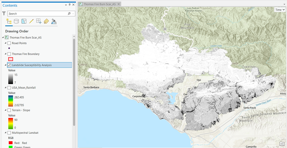
Once I run the processing chain (Figure 7), the final output is generated (Figure 10 below) - the region affected by the Wildfire has been assigned Risk scores ranging from 7 to 15. The higher the scores (whiter pixels), higher the possibility of a Landslide affecting that place.

I hope you were able to appreciate how advanced technology is used to process multiple geospatial data layers into a Landslide Risk Model - the processing happens lightning-quick too. As I never forget to emphasize, the quality of geospatial data is as important as the software's capabilities.
3. Identifying at-Risk Stakeholders & Infrastructure from a Landslide Risk Model

While I had demonstrated the process of creating a Landslide Risk Model in the previous workflow, now I shall use an already-prepared Risk Model over a new study area - Boulder County within Colorado, USA - to identify those stakeholders and infrastructure which are at most risk from Landslides, given a recent wildfire as well as given the fact that the a Landslide is most threatening not at the point of origin but when enough debris accumulate in a steep, downward flow especially after heavy rainfall.
Much thanks to Learn ArcGIS for the training resources
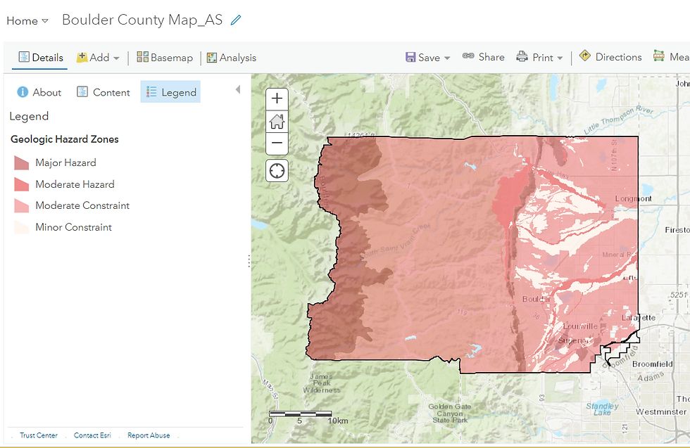


Time for some Analysis.
Let me hover around a few cities falling within the Risk Model's extent....

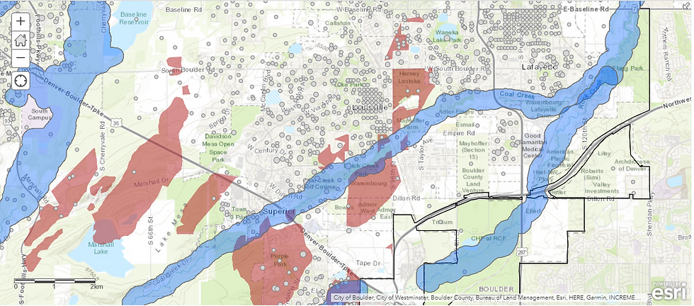
Next, the 'Enrich Layer' geoprocessing tool helps me to add demographic and socio-economic data (acquired by the software developer) to the map. These new geospatial data attributes will help me to analyze the risk in a more in-depth manner.


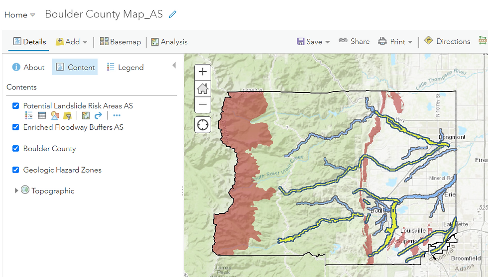
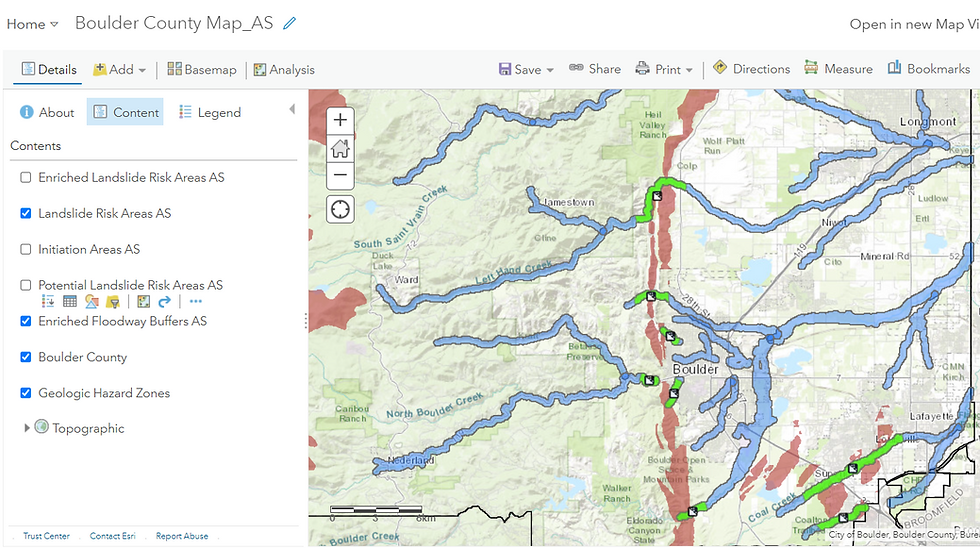
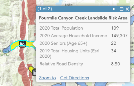
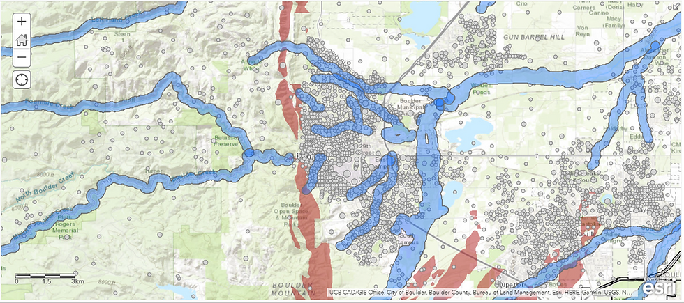
These green zones (Figure 23) are the prime areas of concern. I proceed to enrich this layer with more data. Now, besides Population, I can study other relevant parameters such as Housing units, Property density, Road density, and number of Elderly persons in the highest at-risk areas. This will help the authorities to fine-tune their preventive measures for these zones.
To summarize, GIS helped me to expand the landslide risk model to identify stakeholders and infrastructure at the highest risk.
4. Rapid Detection of Landslide location using Radar Remote Sensing
While the two workflows discussed previously involved the generation of an Early Warning System (EWS) to identify high-Landslide Risk areas and determine the stakeholders and infrastructure who'd be potentially affected, in this third and final workflow, I'll demonstrate how to quickly detect where the Landslide has occurred using Sentinel-1's Synthetic Aperture Radar (SAR) Satellite Imagery.
In the era we live in, one can posit that Landslides are already being detected quickly - footage of flowing debris are quickly captured and circulated in the news and on social media. That being said, knowing the exact location of Landslide initiation and its exact extent is beyond the reach of a common man's handheld device (unless he/she has a Drone 😌). Moreover, many Landslides may not be spotted when there are no human settlements and infrastructure nearby and yet, they are equally necessary to be detected and studied.
Much thanks to RUS Copernicus for the training resources. Processing done on SNAP software
The process of detecting Landslides entails analyzing two SAR Imagery datasets over the same extent and close to each other in terms of timeline - one 'before' the suspected date/time of Landslide and another 'after' it. The next step involves observing discernible changes in the surface features to see if it demonstrates properties indicative of a Landslide - mainly changes in the shape and position of rocks i.e. Deformation.
Radar Imagery has useful characteristics which make it much more advantageous to use over Optical Imagery - it is able to penetrate Cloud cover and can can be acquired even during night-time due to the presence of Microwave Transmitter onboard the Satellite. Optical Imagery, on the other hand, is captured passively - source of illumination being Sunlight - and hence, it can only be acquired during the day-time and atmospheric hindrances such as Cloud cover impact its ability to capture accurate reflectance values of surface features.
The study area for this workflow is Fagraskógarfjall in Iceland where I plan to detect whether and where the Landslide has occured-
I have explained each and every step of this complex processing chain (InSAR Interferometry) in detail in another post - Deformation Mapping for Volcanoes. Hence, in this already long post, I will emphasize only on the most important aspects.

The end-objective of this first part of the processing chain (as depicted in Figure 26 above) is to make the two SAR Satellite Imagery datasets (before & after the suspected Landslide incident) cleaner and comparable. Once the first phase is completed and a Coregistered stack is created (before and after processed Imagery datasets stacked in a single product), I have proceeded to visualize the stack as a RGB composite - it contains information from both the datasets in a single image as seen in Figure 27 below-

There are four colors predominantly - the Yellow pixels denote where both before and after Imagery datasets have the the same reflectance value (Intensity), the Red pixels denote where there is a higher reflectance value in the before Imagery dataset, the Green pixels denote where there is higher reflectance value in the after Imagery dataset and Black pixels denote where there is negligible / zero reflectance value i.e. no data - these are likely to be Water bodies as Water reflects the transmitted microwaves in the opposite direction i.e. away from the Satellite's receiver resulting in negligible / no backscatter received from that surface.
It is the Green pixels that are of particular relevance in this workflow as I will stand to benefit if I know where the surface features have significantly changed in the after Imagery dataset.

The dark green pixels in third image of Figure 27 is indicative that there has been a significant change in the after image from July 2019 - this could be the potential Landslide location and we must inspect it further to validate it.

The next step involves the creation of an Interferogram. This operator enables one to detect and measure the Ground Displacement rate between the pre and post Imagery datasets, with centimeter-level accuracy.
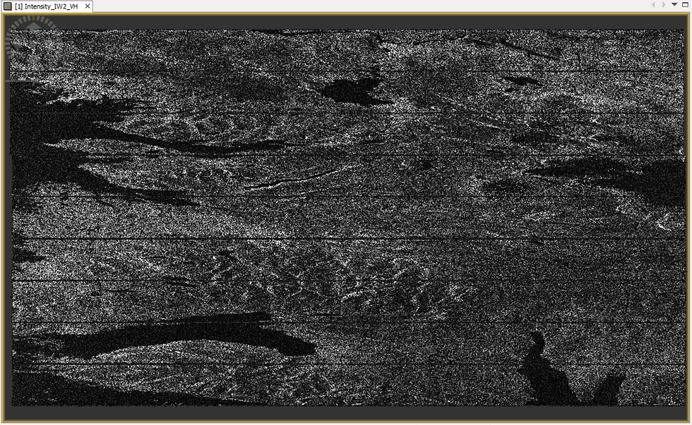
The three outputs generated by this operator are the Intensity, Phase and Coherence bands.
Intensity - In a single Imagery dataset, Intensity means the square of the Amplitude where Amplitude is the microwave energy reflected from the Earth's surface received by the Satellite's receiver. In the Interferogram output, the Intensity band is formed in a slightly different manner - it is derived by multiplying the Amplitude values for the same pixel across both the Imagery datasets within the Coregistered Stack.
Phase - In a single Imagery dataset, Phase is a quantitative value derived using the distance between the satellite's antenna and the ground targets. As I am seeking to measure Displacement (rate of uplift or subsidence), the Phase information and particularly, the change in Phase value becomes vital. The Phase band in the Interferogram output is exactly that - it captures the Phase difference i.e. it is derived by subtracting the Phase value of a pixel in one dataset from the Phase value of the same pixel in the other dataset.
Coherence - Coherence is a measure of Interferogram quality and is a normalized value ranging from 0 to 1 which is derived by combining the Amplitude and Phase values across both the Imagery datasets. If the individual Phase and Amplitude values across both the Imagery datasets are similar, then it signals High coherence (values closer to 1). What a Deformation researcher seeks to closely monitor is zones with Low coherence (values nearer to 0), which indicates that there is a considerable difference in Amplitude and/or Phase values across both the datasets, a telltale sign of Ground Displacement.
What I am essentially trying to do is to compare the change in surface features using in particular the Phase and Coherence information. These will help me to ascertain the presence of Deformation which will validate that a Landslide has occured at that spot.
Besides Landslides, Deformation monitoring is also useful in Earthquake and Volcano workflows.

The loss-of-Phase i.e. a disturbance akin to throwing a pebble in calm, rippling waters as seen on the left in Figure 30 above is indicative of Ground Displacement, a telltale sign of Deformation and in our case, a Landslide.
To explain the 'Coherence' visualization on the right in Figure 30 above, the pixels with very low Coherence values (nearing 0) are Black in color while those with very high Coherence values (nearing 1) are White in color. One can observe a cluster of low Coherence pixels as highlighted in the figure above, it is indicative of a significant shift in surface features between the before and after images. Together with the loss-of-Phase evidence, this strongly points towards the occurrence of a Landslide.
From the Slider below, you can clearly see that the cluster of low Coherence pixels correspond to the known site location of Fagraskógarfjall Landslide in Iceland-
Fascinating, isn't it?
5. Conclusion
To summarize, the Rapid Detection of Landslide location was validated using four observations-
a) Higher Intensity reflectances in the after Satellite Imagery Dataset,
b) RGB Composite of the Coregistered Stack confirming the same (Dark Green pixels),
c) Loss of Phase in the Coregistered Stack, &
d) Low Coherence in the Coregistered Stack
Each of these observations are independently needed to confirm the occurrence of Landslide at that particular location.
Thus, you have witnessed how Remote Sensing helps in the rapid detection of Deformation - strong evidence that a Landslide has occured at that spot. Not only can this procedure be done quickly (processing in SNAP software is a breeze with an industry-grade computer system + the Satellite constellation's revisit time to the same location is also low at ~6 days), it is also cost-effective when compared to Ground-based, Instrument-intensive techniques of landslide detection.
That being said, I had tried to replicate this Landslide Detection workflow on known, recent Indian Landslide sites such as in Mizoram and Kerala states of India. After spending literally several days, my output didn't validate the occurrence of the Landslide at those locations. I suspect Sentinel-1's SAR Imagery works best on large Landslide zones as its spatial resolution is average (1 pixel = 100 sq. m). This in no way is a drawback of the Differential Interferometry technique - rather, I believe that other, higher resolution commercial Radar Imagery satellites would be better suited for the detection of Landslides with a smaller spread. Commercial service providers can direct their Satellite to the study area on-demand so this is an advantage as well in terms of acquiring the after / post-incident Imagery dataset in quick-time.
That being said, one must be wary of Imagery datasets obtained immediately prior and post the Landslide has occured - Landslides are preceded by heavy Rainfall and succeeded by heavy Flooding - Water, as I had mentioned earlier in this post, reflects the Microwave energy transmitted by the Satellite in the opposite direction i.e. away from its receiver. Therefore, both the before and after Imagery datasets would show very low reflectance values in the pixels where the Landslide has occured. This would hamper the accurate detection of Landslide because the methodology of Differential Interferometry for Deformation is based on detecting significant change in reflectances over the same surface feature over two or more time periods. I think this is the reason why my analysis for Mizoram and Kerala Landslides was not successful - both the regions are prone to heavy-rainfall virtually throughout the year and therefore, my selection of the before-incident Imagery hampered a positive outcome. Difficult to know when those locations had a continuous spell of no-rain days which would be ideal to obtain an Imagery dataset!
Hope you enjoyed the Landslide Hazard Mapping Workflows on Risk Modeling, Analysis & Detection covered in this post.
ABOUT US
Intelloc Mapping Services, Kolkata | Mapmyops.com offers Mapping services that can be integrated with Operations Planning, Design and Audit workflows. These include but are not limited to Drone Services, Subsurface Mapping Services, Location Analytics & App Development, Supply Chain Services, Remote Sensing Services and Wastewater Treatment. The services can be rendered pan-India and will aid your organization to meet its stated objectives pertaining to Operational Excellence, Sustainability and Growth.
Broadly, the firm's area of expertise can be split into two categories - Geographic Mapping and Operations Mapping. The Infographic below highlights our capabilities-

Our Mapping for Operations-themed workflow demonstrations can be accessed from the firm's Website / YouTube Channel and an overview can be obtained from this brochure. Happy to address queries and respond to documented requirements. Custom Demonstration, Training & Trials are facilitated only on a paid-basis. Looking forward to being of service.
Regards,

